Author’s note: This is my first entry in The Neuroverse, and the main reason why I started to take self-learning seriously… There’s only so many times I can pretend to know what a Morlet wavelet is.
Time-frequency analysis is a signal processing technique that evaluates how oscillatory brain activity changes over time at different frequencies, rather than looking at the time or frequency domains separately.
To understand where this method comes from, and why it’s needed, it helps to start with the operation it’s built on: the Fourier transform.
The Fourier Transform
In a Fourier transform (FT), we decompose a signal that varies over time into its component sine waves to find out how much of each frequency is present. In other words, it determines the extent to which each frequency contributes to the original signal.
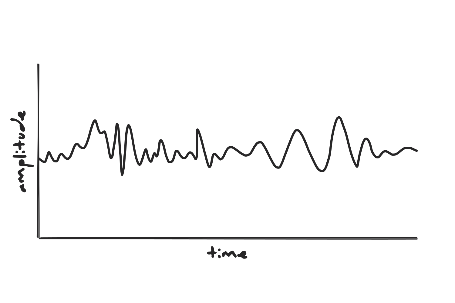
Comparing frequencies
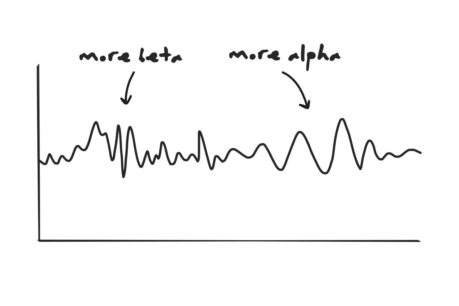
We can apply a Fourier transform to find how much the signal above resembles a sine wave at each different frequency. In each of the two images below, we see our signal and an overlapping sine wave: the first one corresponds to alpha oscillations, and the second one to beta oscillations. The closer a sine wave matches the ups and downs of the signal, the more power that frequency is assigned.
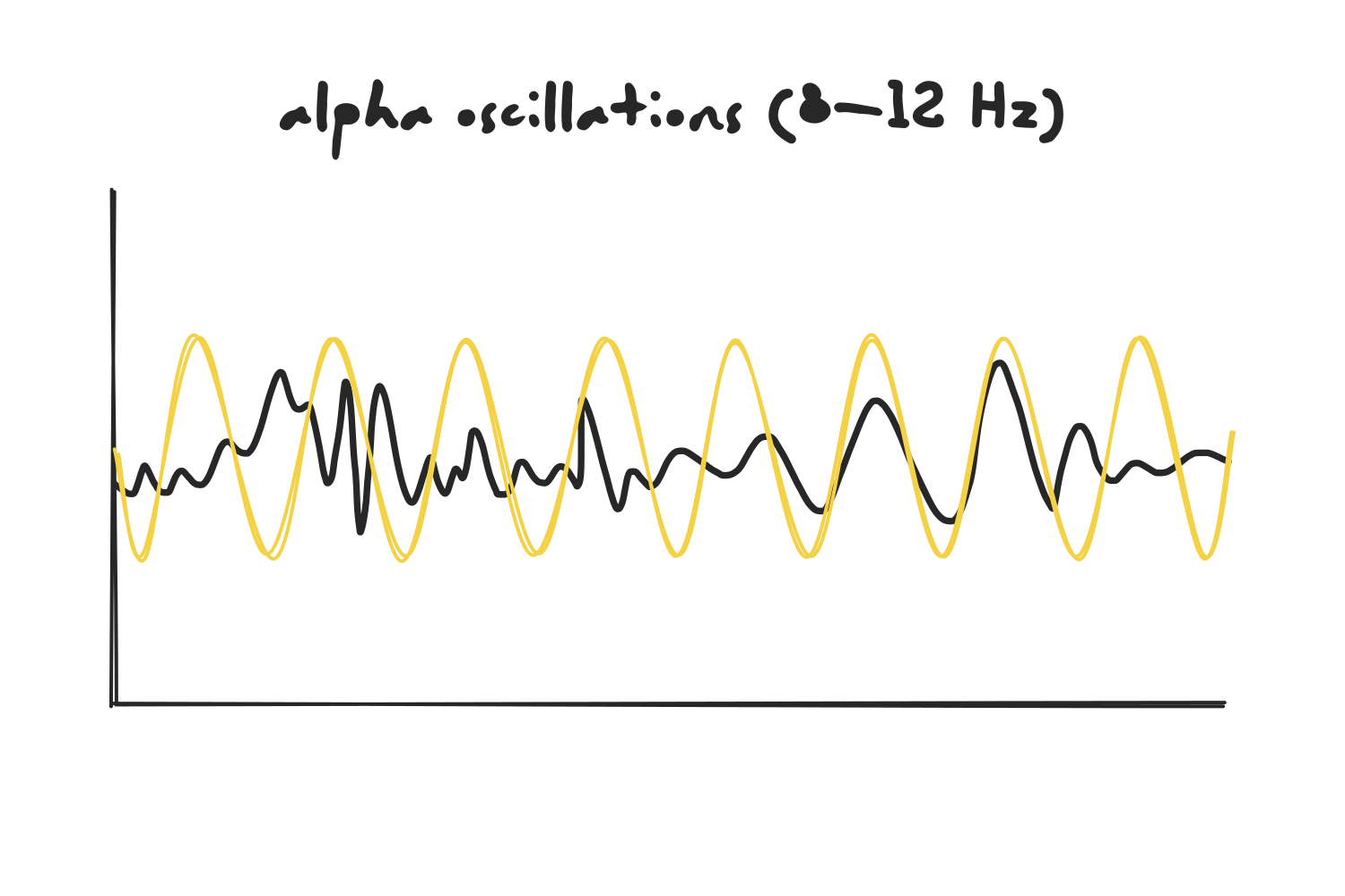
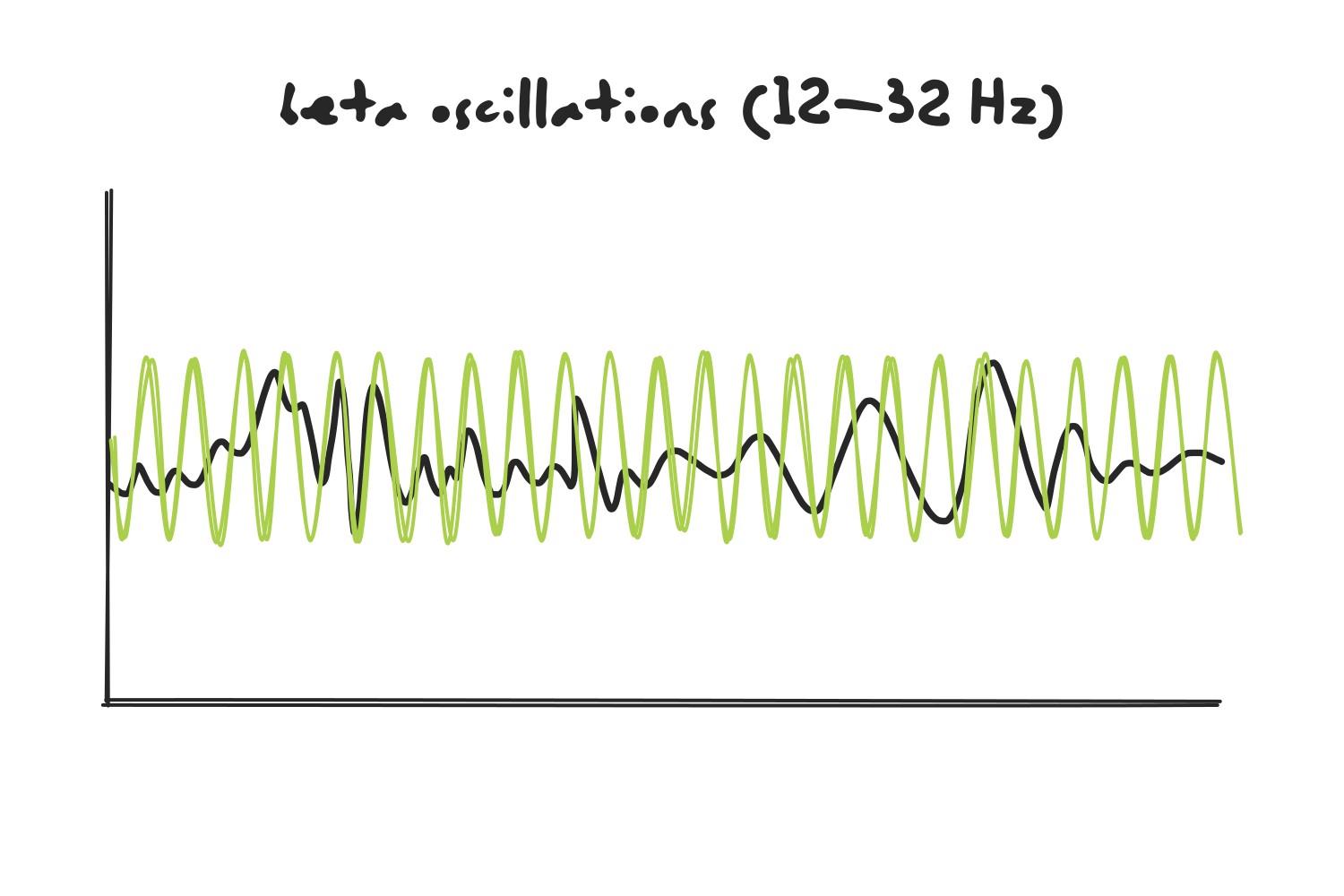
(Note that a real Fourier transform treats each frequency separately, so instead of comparing the signal to an alpha oscillation, it is compared to sine waves at 8 Hz, 9 Hz, 10 Hz, and so on. I’m grouping them into bands here to keep the picture simple.)
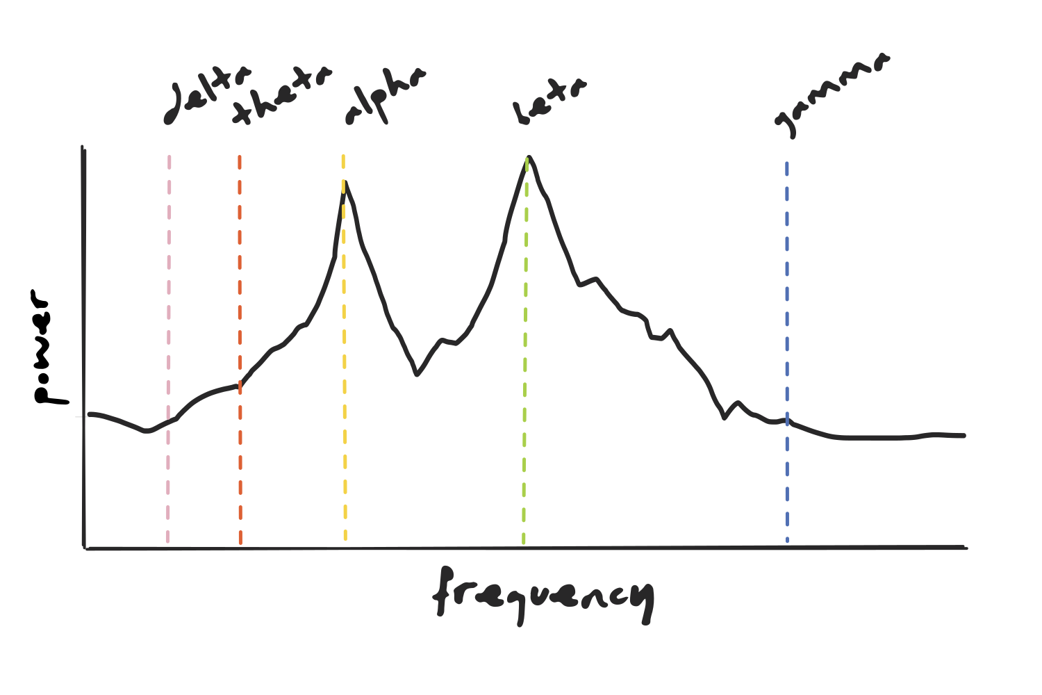
Repeating this across all frequencies gives us the power of each frequency within the whole signal, which we can visualize as a frequency-power plot.
Continuous vs. Discrete
Before going further, let’s understand one technical detail: the classical operation (also known as the Continuous Fourier Transform) is defined as an integral over a continuous signal of infinite duration, so we can’t run it on a computer, which is only able to handle discrete, finite data. The solution is the Discrete Fourier Transform (DFT), a version of the operation that takes a finite number of evenly sampled points and returns a finite number of frequencies. Computing a DFT directly is slow, so in practice we use the Fast Fourier Transform (FFT), an algorithm that produces exactly the same result but far more efficiently. The two terms are often used interchangeably, but strictly speaking, the DFT is the operation and the FFT is the shortcut used to compute it.
The time limitation
Now, back to the spectrum itself. Since each frequency is summed over the entire time window, it ends up with a single power value and all temporal information is lost. In the case of our signal, there is more beta activity at the beginning and more alpha activity towards the end, but this would go unnoticed.
The Short-Time Fourier Transform
To keep temporal information, we turn to another method derived from the same mathematical operation. The Short-Time Fourier Transform (STFT) chops the signal into shorter segments using a window that slides along the entire signal and computes the FFT at each position.
Each segment yields its own power spectrum, which only describes the signal over that specific time window. Stitching them together in chronological order creates a spectrogram, in which the x-axis corresponds to time, the y-axis to frequency, and power is represented by color. The shift from beta to alpha that the power spectrum concealed is now visible, and we can see two distinct components.
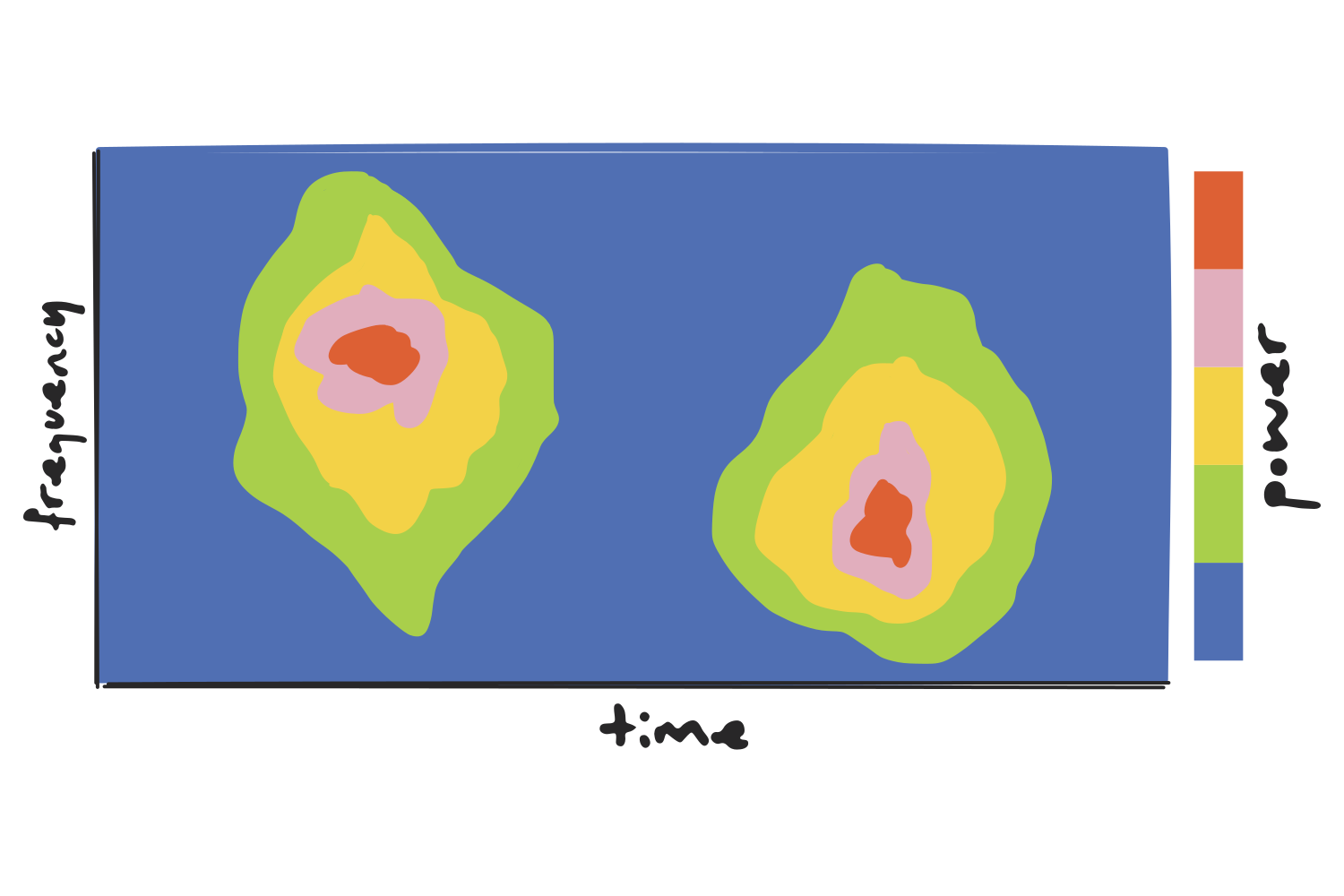
(A real spectrogram is a continuous heatmap, much noisier than the one shown above. The blobs here are just meant to illustrate the idea more clearly: hot regions mean high power at that frequency, at that moment.)
The resolution trade-off
Still, the STFT is limited by its fixed window size: wider windows mean better frequency resolution but poor time resolution, while the opposite is true for narrower windows. Since the same window is applied to the entire signal, every frequency ends up analyzed at the same resolution, regardless of whether that suits it.
Let’s take a one-second window as an example and apply it to two different observations.
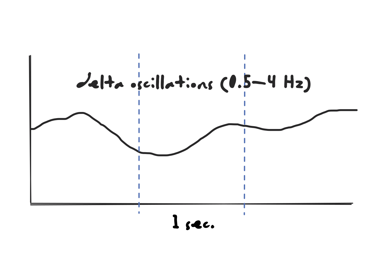
On one hand, the window would be too short for the slowest oscillations in the delta range. A 0.5 Hz wave takes two full seconds to complete a single cycle, so a one-second window never contains a whole oscillation, and the pattern would not be recognized.
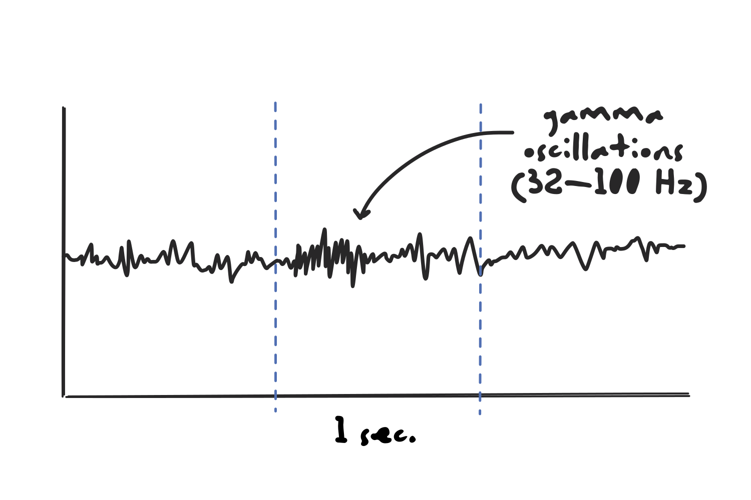
At the same time, the window would be too long to capture the exact timing of high frequency activity such as gamma oscillations. A burst lasting a few tens of milliseconds would be averaged across the entire second, completely blurring out when it happened.
The Wavelet Transform
The solution to the fixed-window problem is the wavelet transform, in which the signal is not compared to an infinite sine wave but to localized wave-like oscillations.
There are different types of wavelets, but the most common for time-frequency analysis are Morlet wavelets, which are created by multiplying a complex sine wave by a Gaussian window.
(Warning: A bunch of math-related stuff coming up next. I tried to jump ahead of these concepts thinking that they were beyond the scope of what I am trying to do, but then I found myself asking important questions that brought me back. The initial “Ugh…” only lasted a few minutes though, and I actually found these ideas to be very interesting once I was able to visualize the concept in my head.)
The complex sine wave
A complex sine wave can be imagined as a 3D shape resembling a corkscrew, and it is used instead of a simple, flat sine wave because it has no blind spots. If we were to use a 2D sine wave to detect a frequency, the answer we get would depend on how the signal happens to line up with it.
To understand this, we need to look at what “comparing” a signal to a sine wave actually involves: we multiply the two point by point, then add up the result across time. This calculation is called a dot product, and it shrinks the whole comparison into a single number for that frequency.
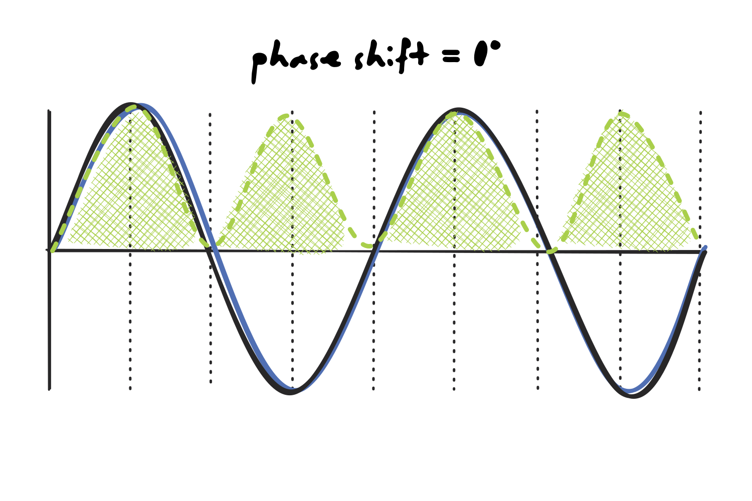
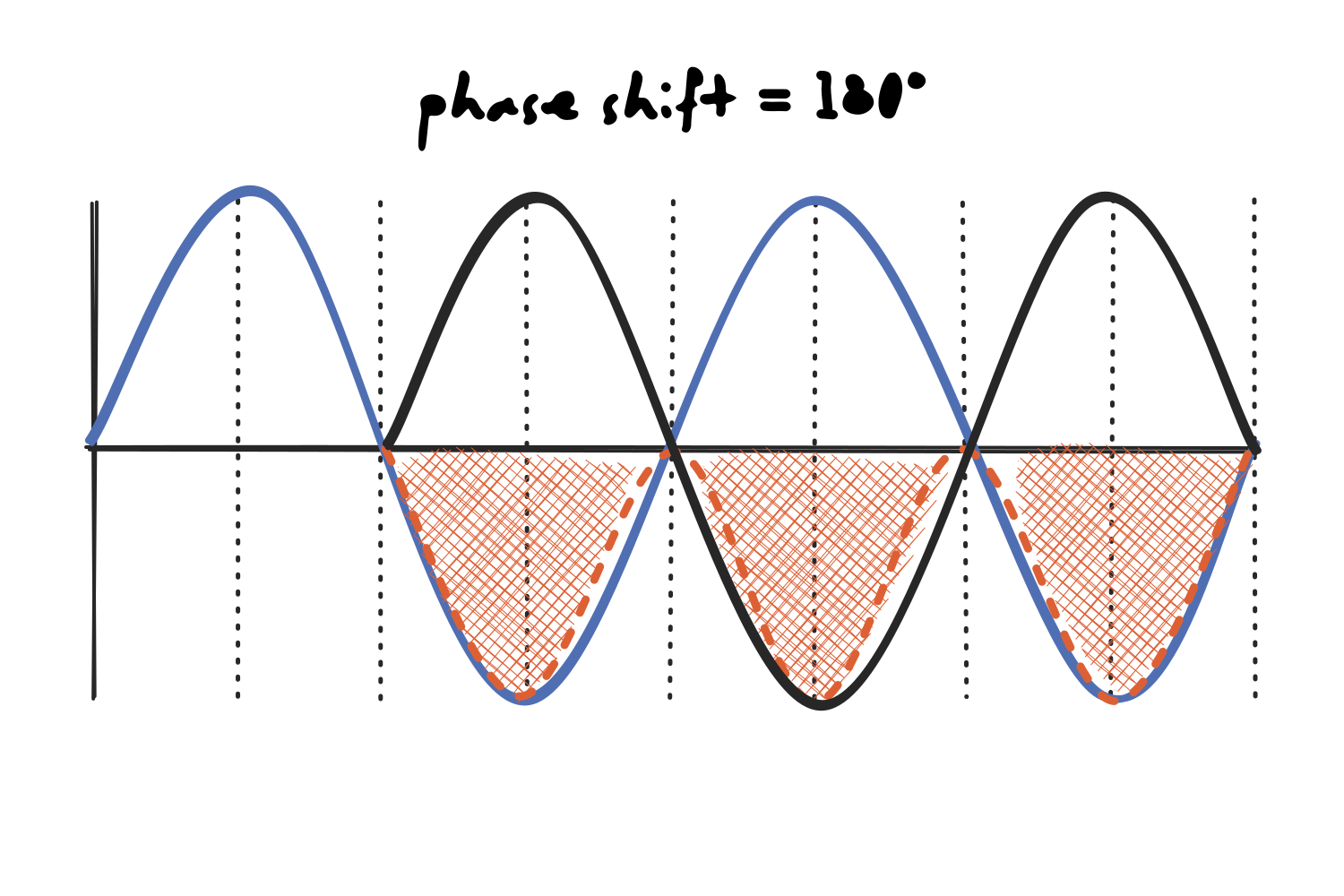
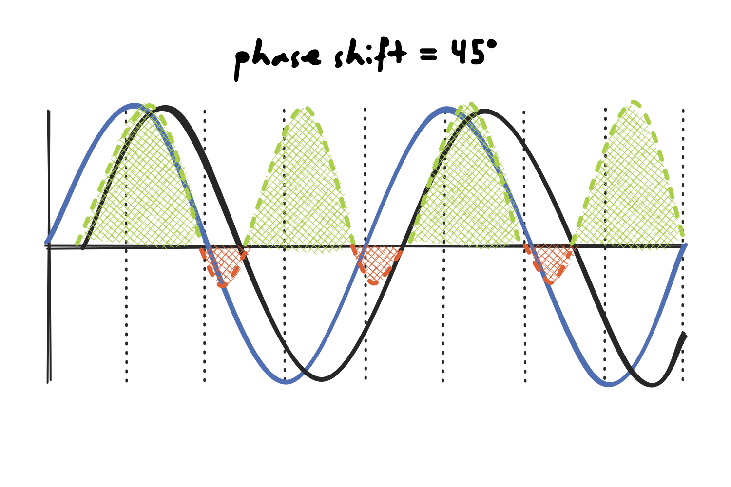
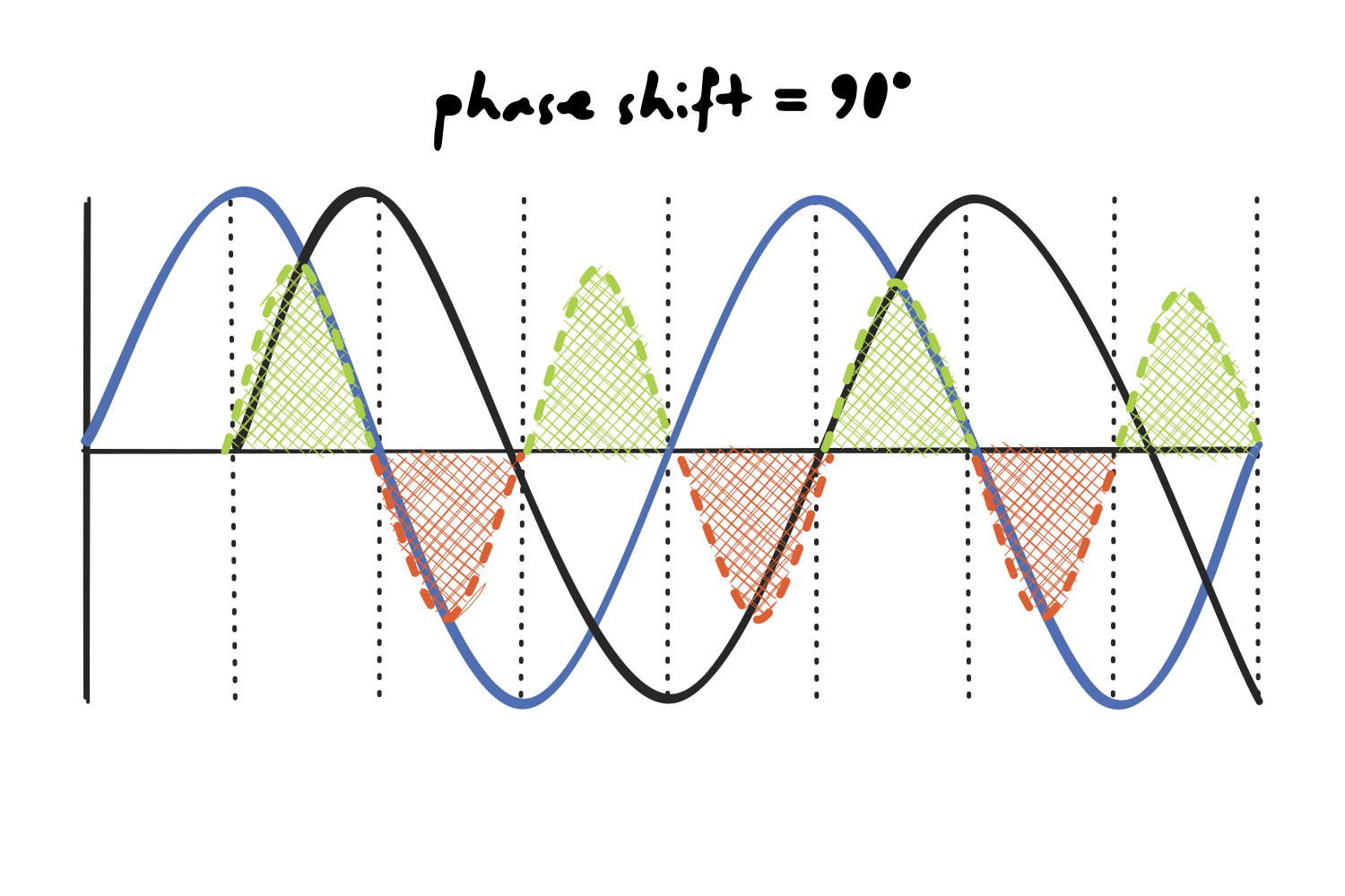
In the images below, the black line is our signal and the blue line is the sine wave we are comparing it to. The shaded region is their product (green where it is positive, orange where it is negative).
Let’s start with a signal that lines up perfectly with the sine wave. Both waves are positive and negative at the same moments, so their product is positive everywhere. The area is entirely green, so we know that the score is a relatively large and positive number, and the frequency is correctly identified as having high power within the signal.
Now let’s take a look at the opposite case, where the signal is flipped with respect to the sine wave. Every time one wave is positive the other is negative, so the product is negative everywhere. However, since we only care about how much of the frequency is present and not its direction, we take the magnitude of that score and ignore the sign, so the power would be identical to the case above.
In between these two extremes, the product splits into positive and negative areas. At a 45° shift, the green area still outweighs the orange, so we are left with a net positive score, but by a noticeably smaller margin than at 0° or 180°, even though the signal contains exactly the same amount of that frequency.
The number we get depends on how the two waves happen to line up, but at a 90° phase shift, when the signal is a quarter of a cycle out of step with the sine wave, the positive and negative areas are equal, so they cancel out to zero and make it look as if that specific frequency was not present at all.
Now that we understand the issue, we can see how a complex sine wave solves it: it carries two waves at once rather than one.
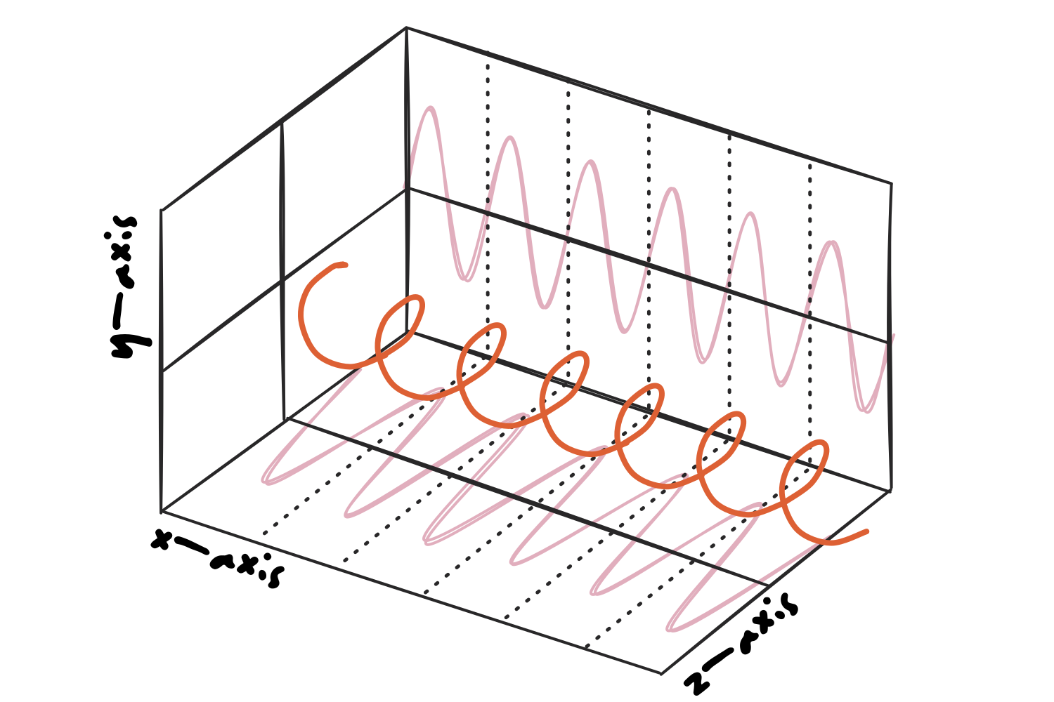
Those two waves are a cosine and a sine of the same frequency, which are the same shape shifted by exactly a quarter of a cycle: whenever one of them is passing through zero, the other is at its peak. Therefore, the blind spot of one is always covered by the other.
(Note that complex sine waves are also used in Fourier transforms, but this explanation was omitted before because we’re learning one thing at a time.)
The Morlet wavelet
So, this complex sine wave is multiplied by a Gaussian window (which is shaped as a bell curve) to create a Morlet wavelet that tapers off to zero on both ends.
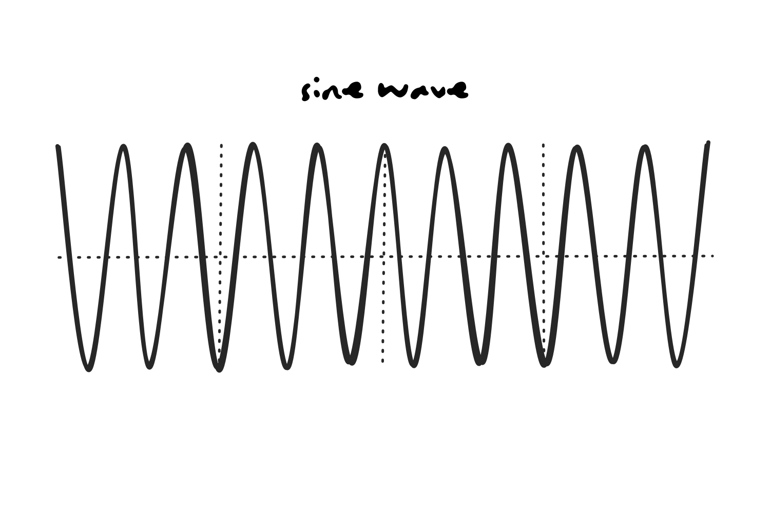
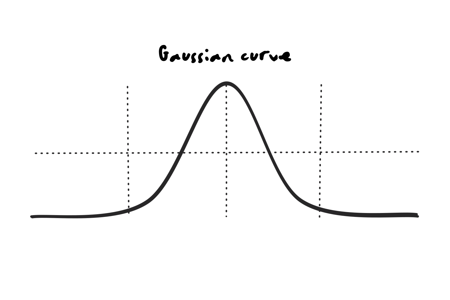
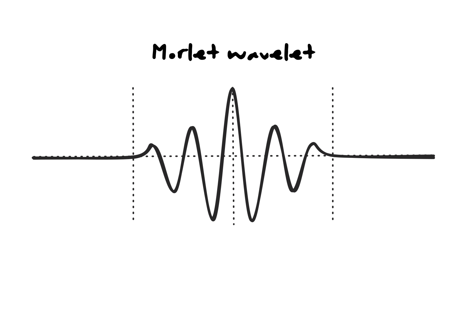
We do this to prevent spectral leakage, a phenomenon that introduces artificial frequency artifacts when a sine wave is cut off abruptly.
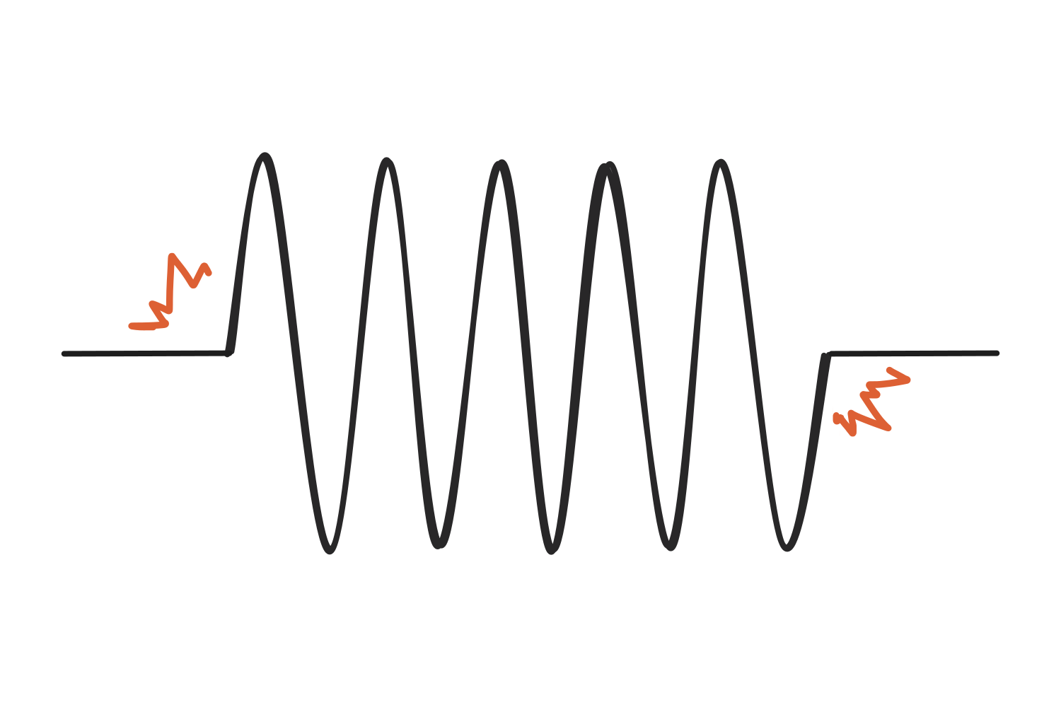
Since a sharp edge is not something any single frequency can produce on its own, reproducing it requires adding power at many other frequencies, and the chopped wave ends up leaking additional power across the spectrum instead of representing one clean frequency. Tapering the ends removes the edges and keeps the estimate clean.
Convolution
Now, when using a wavelet instead of a sine wave to analyze the distribution of frequencies within a signal, we calculate the product of the signal and the wavelet at each timepoint, then add them together (yup, dot product!) and assign the result to the time point that lines up with the center of the wavelet. In the image below, the black line at the top is our signal, the green one underneath is the wavelet, and the blue dot at the bottom is the single number that comes out of that comparison.
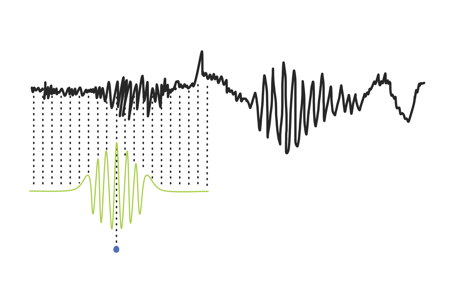
Then, the wavelet slides over to the next time point and the steps are repeated, over and over, until it has covered the entire signal. Every score gets plotted in blue underneath, and together they trace out the line we see below: our result.
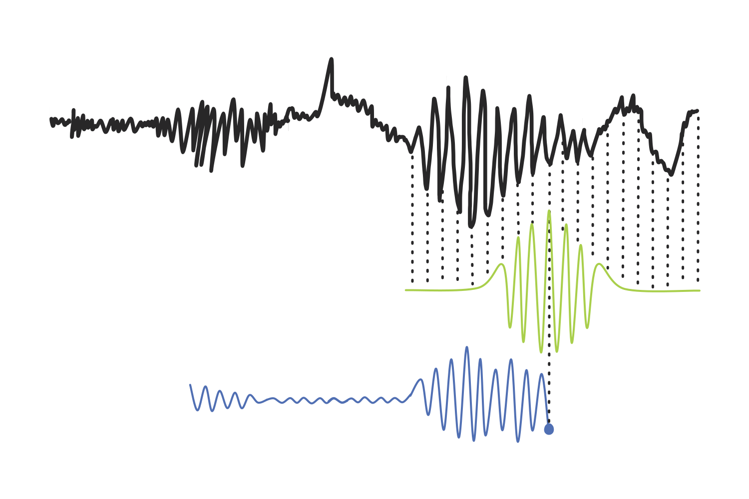
This process in which two signals are blended to produce a third one is called a convolution, and the signal that acts as the filter (in our case, the Morlet wavelet) is known as a kernel.
Edge effects and zero padding
There is one issue that needs to be addressed: if the first product is plotted in line with the center of the first wavelet, the result has no values for any of the samples before that point, and none after the center of the last wavelet either. The output ends up shorter than the signal, missing half a kernel at each end, and the features sitting at those edges are lost.
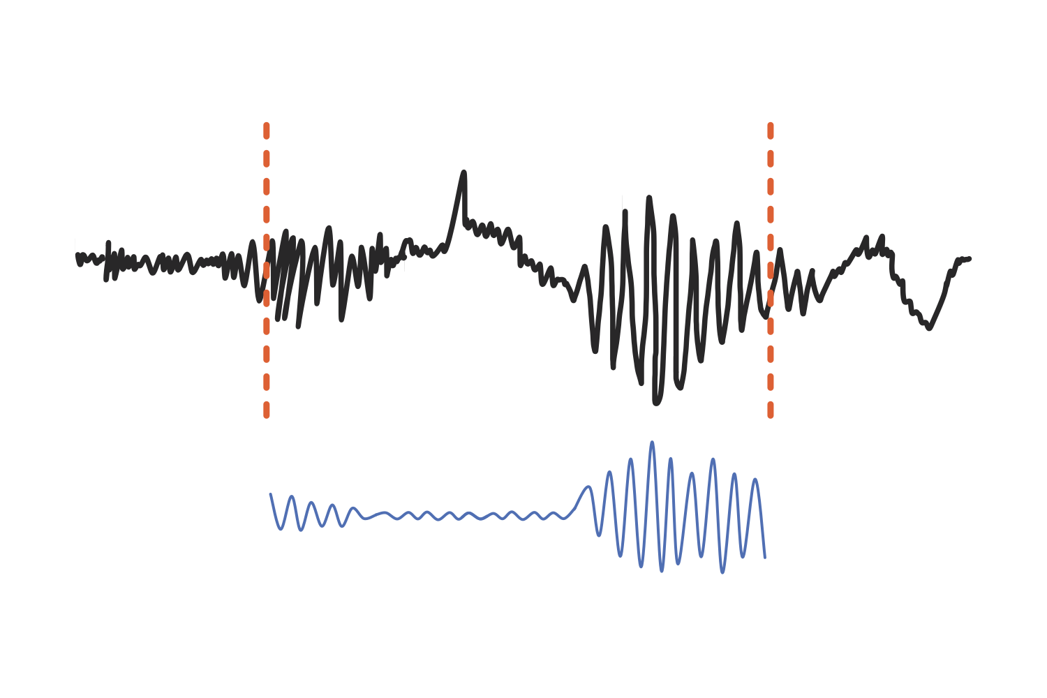
To avoid this, we slide the wavelet back so that it begins before the signal does. Instead of the two starts lining up, the last sample of the first wavelet is aligned with the first sample of the signal.
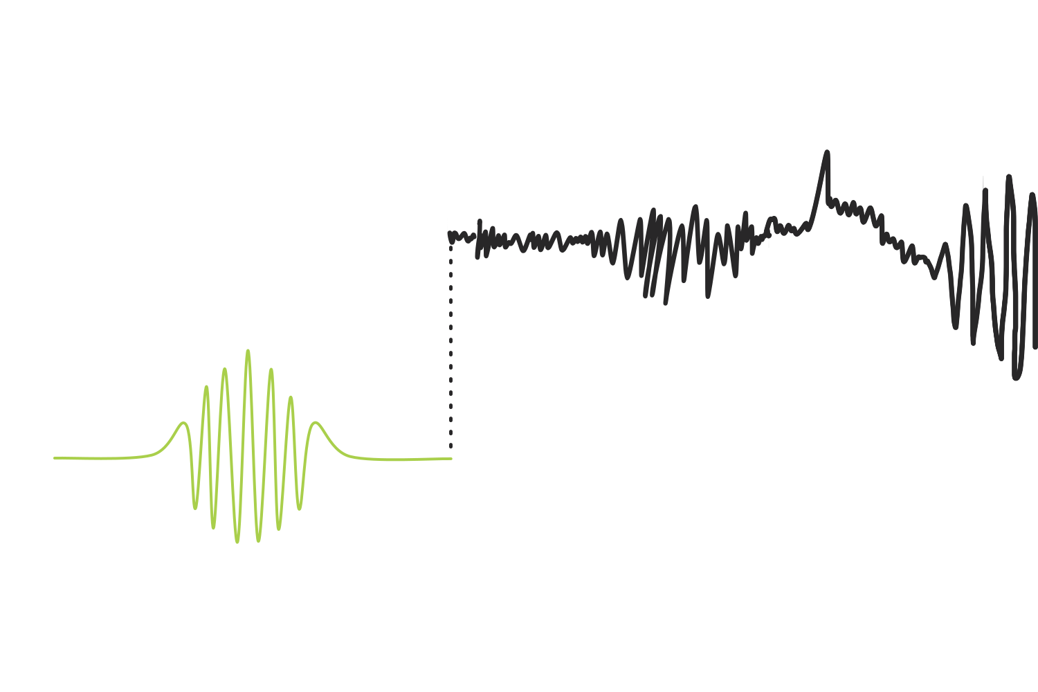
However, this introduces another issue where the rest of the kernel is left hanging off the edge. The fix is a technique called zero padding, where the signal is extended by adding zeros so that the convolution can be completed.
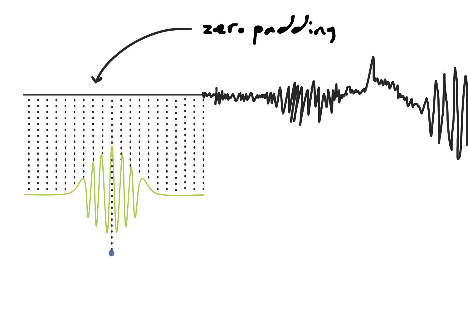
The same problem shows up at the other end. Once the wavelet reaches the last samples of the signal, half of the kernel is hanging off the right edge instead of the left, so we pad that side too and let the convolution run until the first sample of the kernel meets the last sample of the signal.
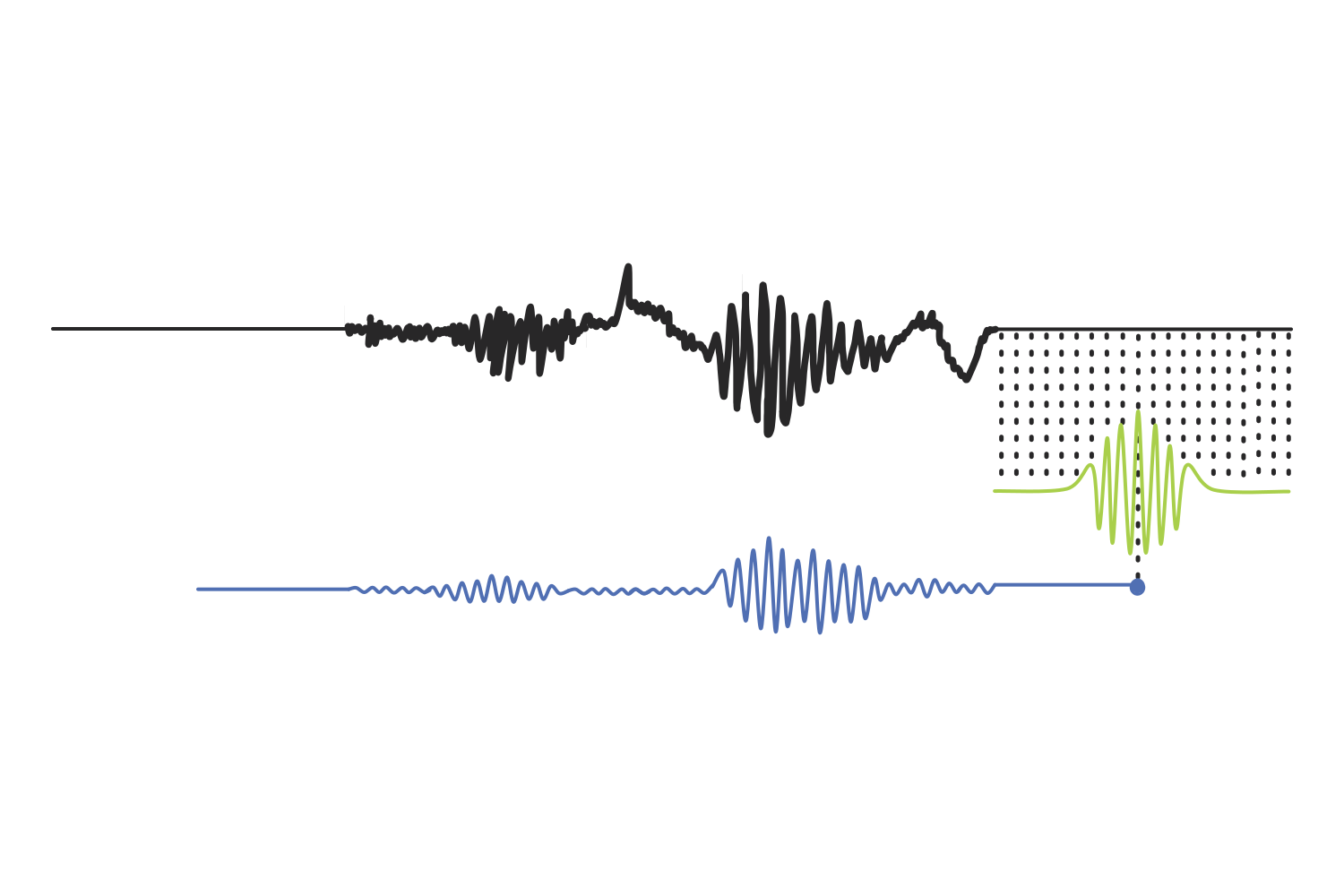
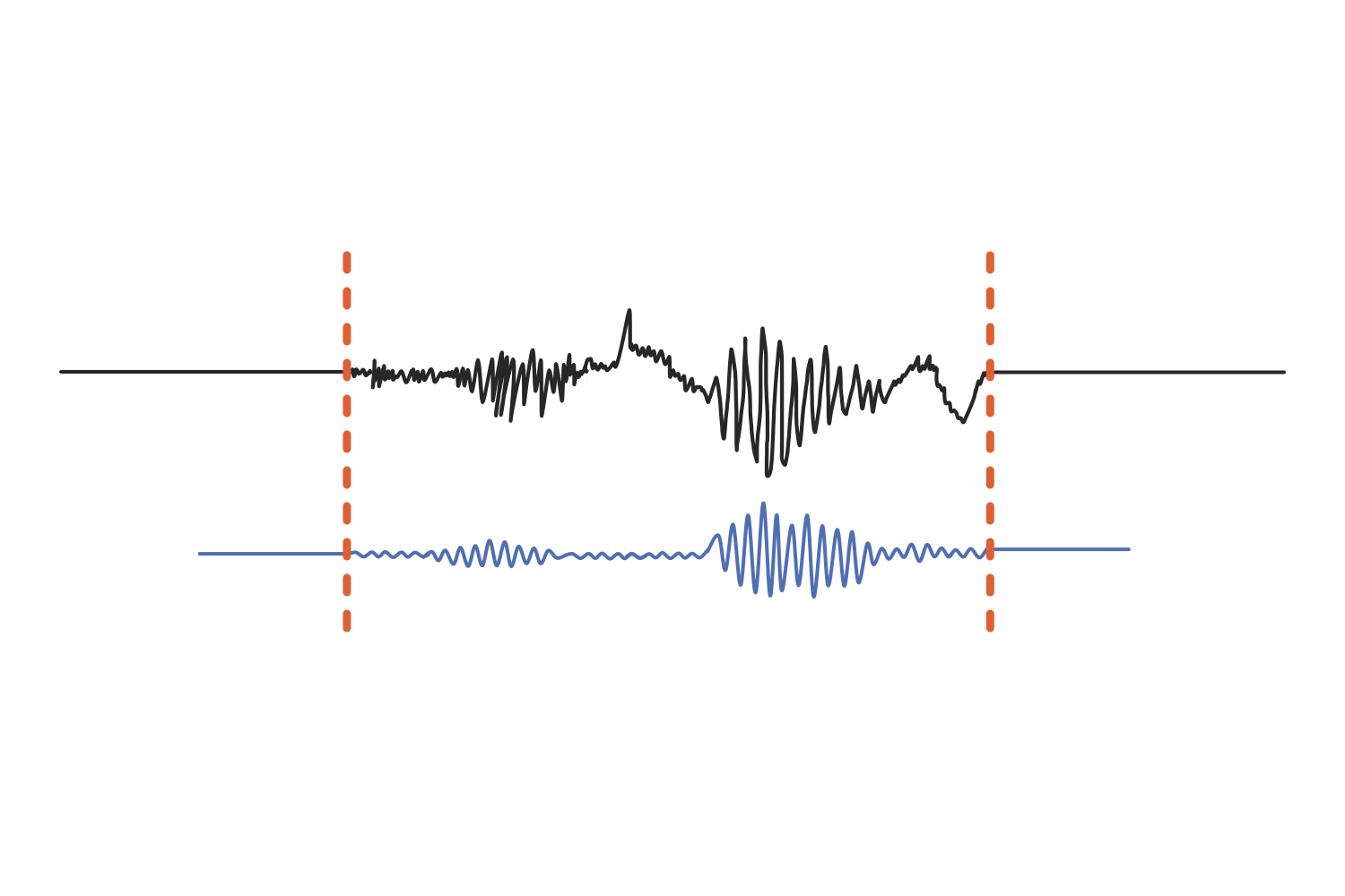
The artificial “wings” at both extremes are discarded once the operation is over, and we are left with a result that is the same length as the original signal.
Wavelet coefficients
Now, let’s take a step back: since we used a complex sine wave to create the Morlet wavelet, that means the wavelet is also complex, meaning that it also carries two waves (sine and cosine) at once. Following this same logic, since the kernel in our convolution is a complex signal, each dot product in the result of convolution is also a complex number, and it is referred to as a wavelet coefficient.
(In mathematics, “complex” means that the value or shape has a real part and an imaginary part. However, for someone like me whose native language is not math, I initially found it easier to visualize the mysterious imaginary part as adding another dimension. For example, just like we imagined our complex sine wave as a corkscrew, a complex Morlet wavelet sort of resembles the ball inside a protein shaker bottle… I know, weird analogy, but they both have the same spiralling spring shape.)
This distinction is important because a complex number carries two quantities at once: a magnitude and an angle. The magnitude gives us the amplitude of that frequency at that moment (and therefore the power, which is equal to the square of the amplitude), and the angle gives us its phase. The frequency itself is not something we extract from the coefficient, but we already know it since it is the frequency of the sine wave we built the wavelet from.
In order to extract all that information from a complex number, we must learn about Euler’s formula, which tells us that any complex number can be expressed as where (for radius) is the distance from the origin, is the angle measured from the positive real axis, is a constant approximately equal to 2.71828 (Euler’s number), and is the imaginary unit (the square root of -1).
This is easier to visualize as a plot than it is to read, so let’s examine what a wavelet coefficient would tell us from looking at it in a 2D complex plane.
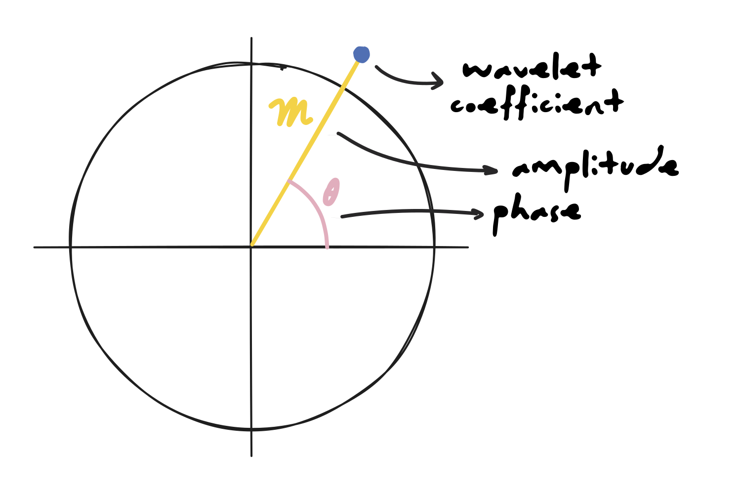
(In the context of signal processing, is often written as because the formula is adapted to represent magnitude, so the form is written as .)
Building the spectrogram
Now we have everything we need to place a single point on a spectrogram. On the x-axis goes the time point corresponding to the center of the kernel, and on the y-axis goes the frequency of the sine wave used to create the Morlet wavelet. Both of those we knew already. What the coefficient adds is the value at that intersection: the color, given by the power we just calculated out of its magnitude.
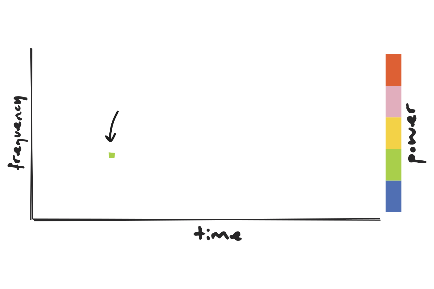
If we repeat this process for every timepoint at every frequency, we get a clear picture of the distribution of different frequencies in our signal and how they change over time…
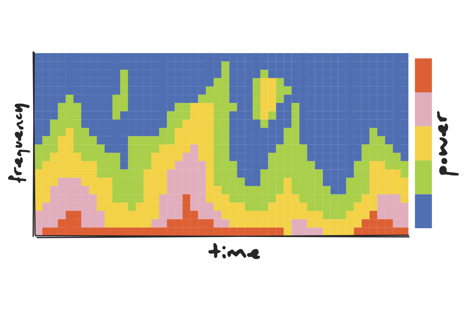
…and that’s what you call a time-frequency power plot!
(We can also generate a time-frequency phase plot if, instead of taking the magnitude of each coefficient, we take its angle. The layout stays exactly the same, with time on the x-axis and frequency on the y-axis, but the color would tell us where in its cycle each oscillation was at that moment, rather than how strong it was.)
The Gaussian width
When talking about the construction of a Morlet wavelet, there is one bit that we skipped over, and it just so happens to be the most important detail in the whole method (which is why I saved it for last): the width of the Gaussian curve that tapers the wavelet.
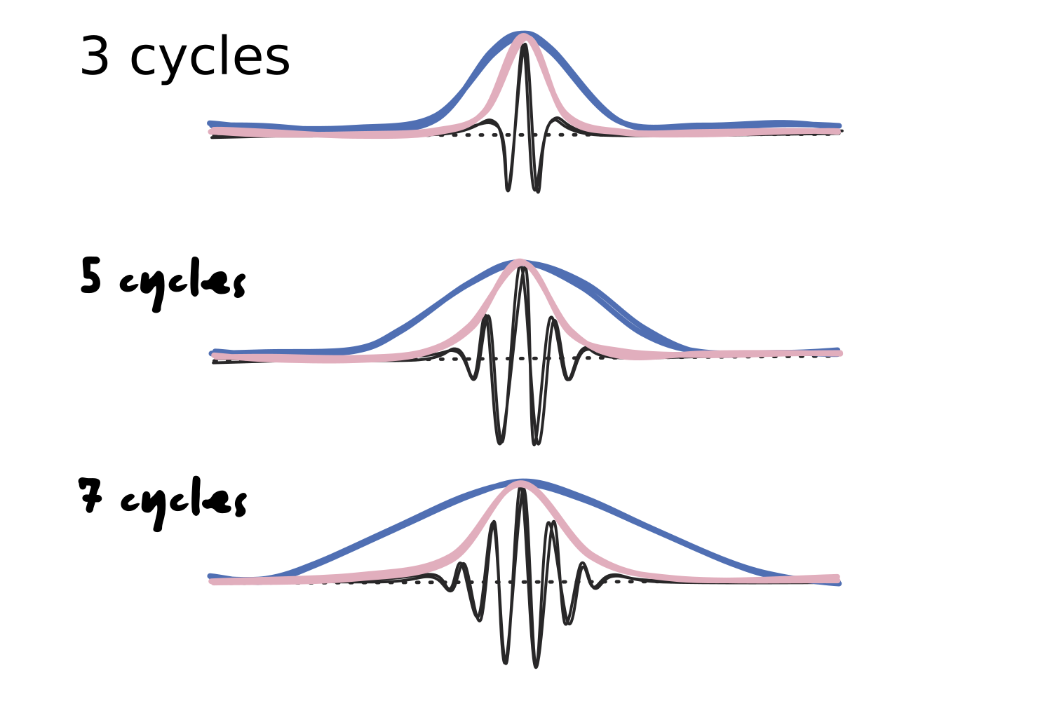
This parameter is not defined by a specific time duration, but rather by the number of cycles of the sine wave that should fit in it. As the number of cycles increases, so does the width of the window.
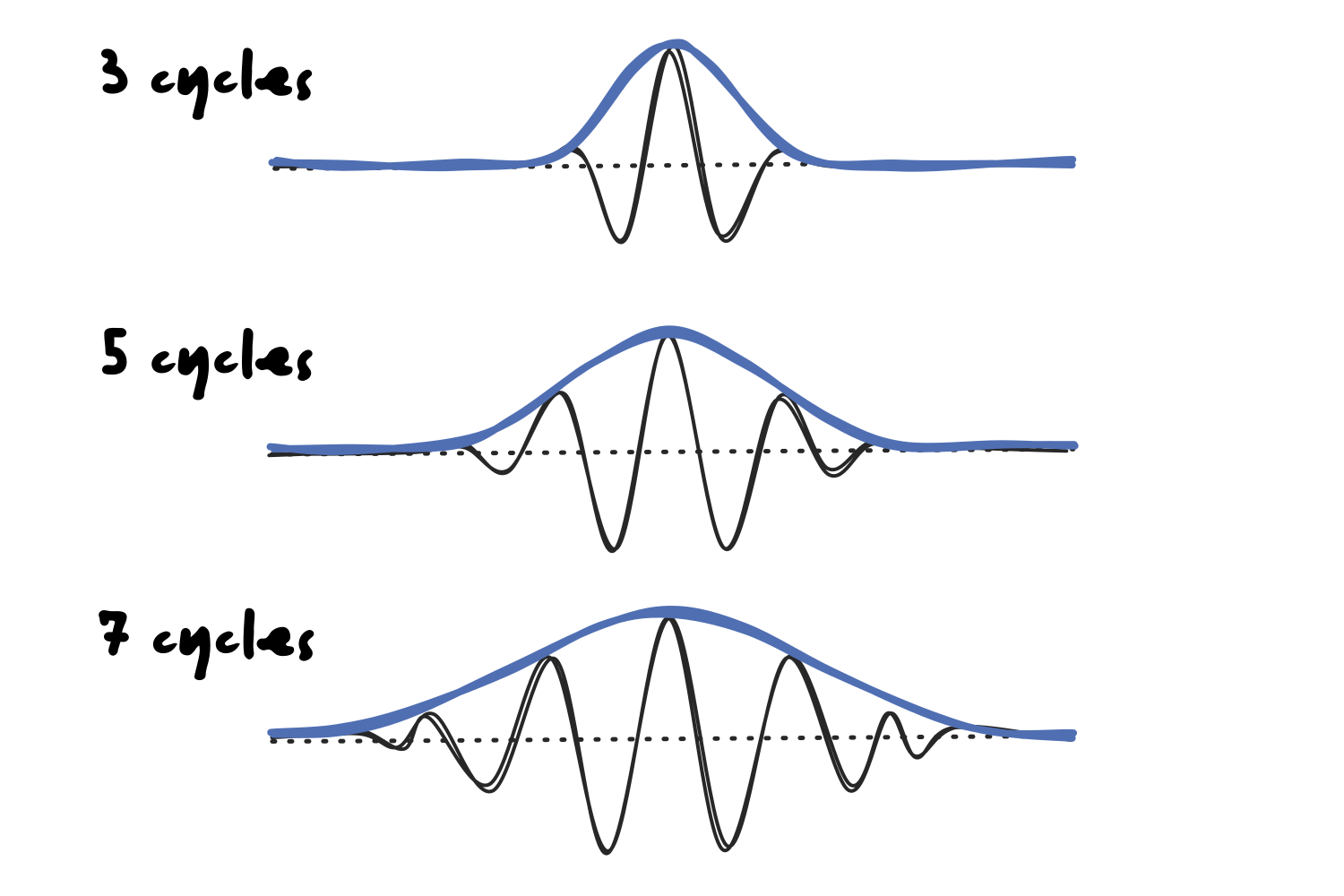
The width of the curve is also dependent on the frequency of the sine wave, since a higher frequency will fit the same number of cycles in a more narrow curve.
Let’s recall the issue that we ran into with the STFT, where a one-second window was too short to identify the frequency of slower waves but too long to detect the exact timing of faster ones. That constraint is called the Gabor limit, and it states that a signal cannot be sharply localized in both time and frequency at the same time.
Morlet wavelets are not an exception to this rule, but they do handle it more efficiently. However, before we dive deeper into the solution, it’s worth taking some time to fully understand the time-frequency trade-off dilemma.
First, let’s assess how the width of the Gaussian would affect the convolution operation. Specifically, we are talking about convolution in the time-domain, since the kernel slides along the time series.
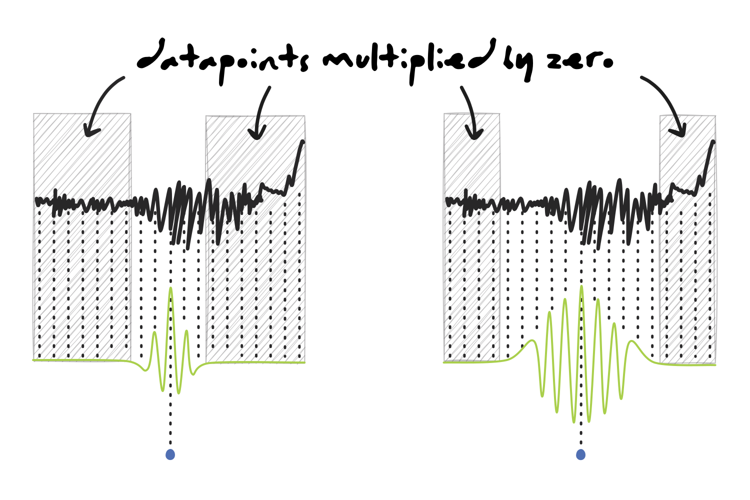
Using a narrow wavelet would give us better temporal resolution because most of the signal would be multiplied by zero, and only the data points in a relatively small area surrounding the center of the kernel would actually be included in the calculation. This means that the result of the dot product is highly representative of the activity at that specific time.
On the other hand, as the wavelet gets wider, there are less points with a value of zero, which means that the dot product is influenced by a longer section of the signal and not as precise in terms of timing.
Judging by that, we would be inclined to think that making our wavelet as narrow as possible would give us the best temporal representation of the signal, which is one of the most important characteristics of EEG data. Unfortunately, when shifting from the time domain to the frequency domain, the situation changes.
A few paragraphs earlier, we learnt about spectral leakage and discovered that the reason behind tapering a sine wave is to avoid cutting it off abruptly and creating a sharp edge, which would require adding power at many other frequencies that would smear our spectrum. Now is the time to take that explanation one step further.
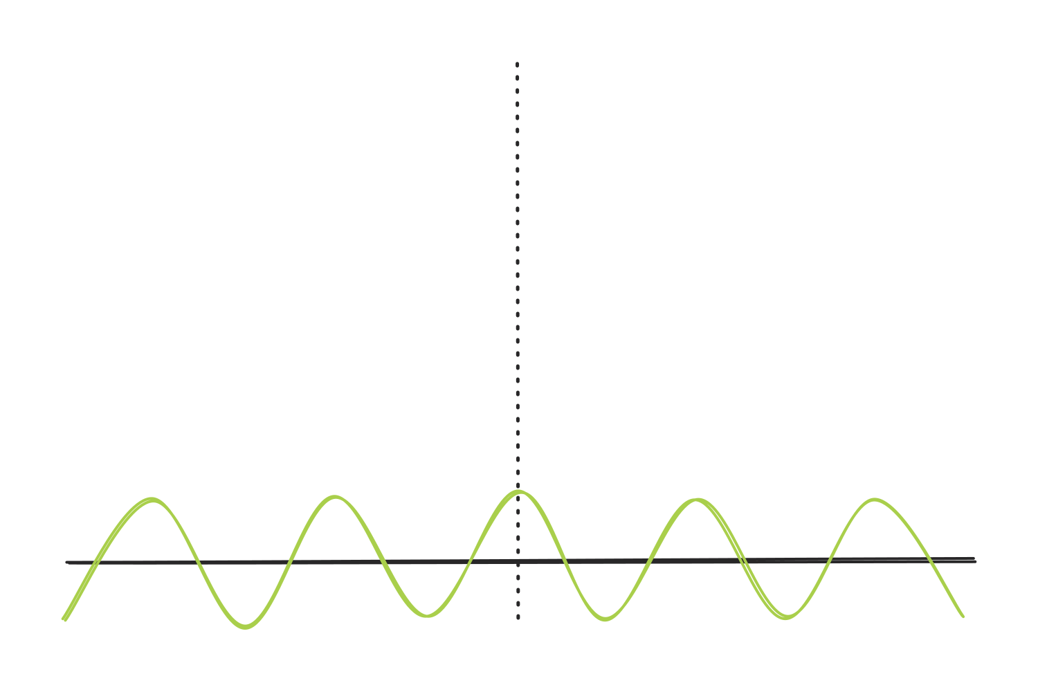
Let’s visualize a wave of some frequency.
Now, let’s add a wave of a higher frequency and align them so they both hit a peak at the same time.
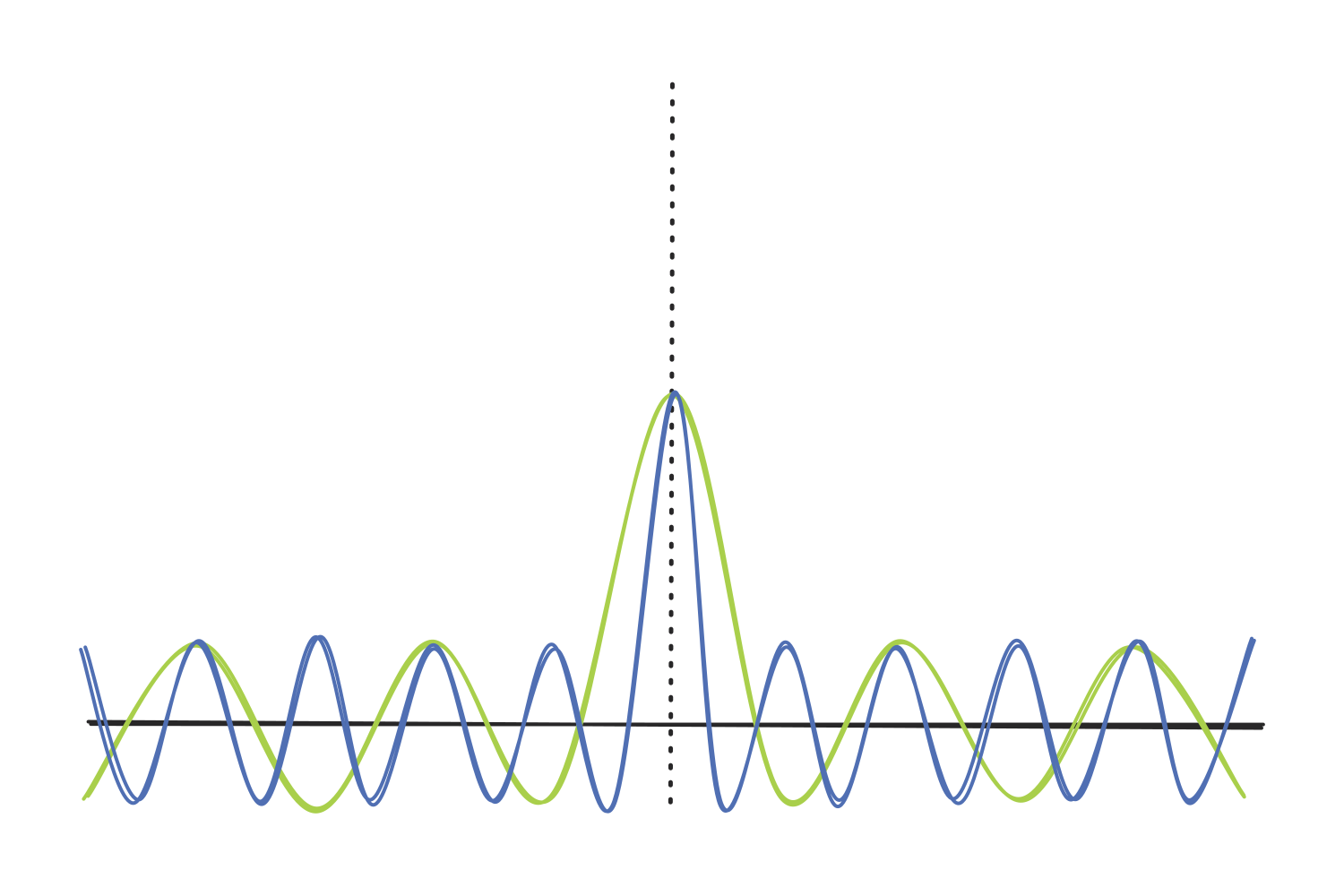
The two peaks add together in terms of amplitude, creating a taller, sharper spike. However, as the waves move away from it, they fall out of sync. As one goes up and the other one goes down, they cancel some of each other out.
The more frequencies we add, the sharper the effect becomes.
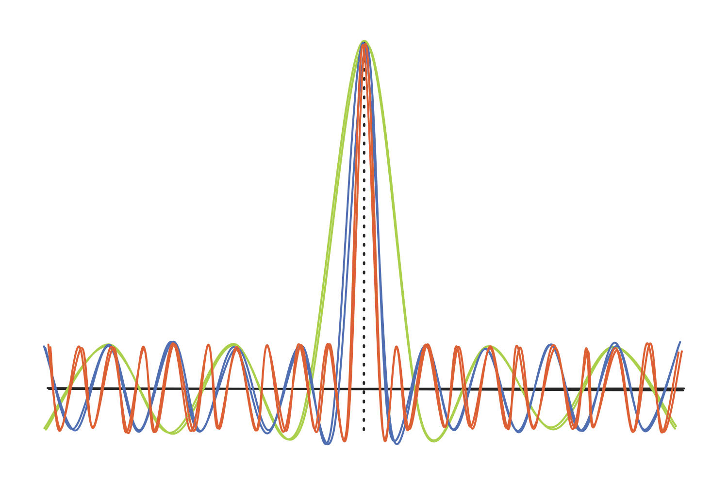
We can repeat this process with every possible frequency, all perfectly aligned to peak at the same time. The result would be an infinitely thin spike of infinite amplitude, and everything else would be equal to zero.
(You might think “Okay, but what about a 100 Hz sine wave? Its peaks are much sharper than, let’s say, a 5 Hz sine wave, yet it only consists of one frequency: 100 Hz.” Yes, that is correct, but the catch is that a sine wave is continuous. Adding many other frequencies is just how we isolate the peak by canceling out the rest of the wave, which is also known as destructive interference.)
Going back to our wavelets, this becomes a problem: the steeper the Gaussian curve in the time domain, the more frequencies needed to produce it. Therefore, if we use a narrow wavelet as a kernel, it will contain and be sensitive to a range of frequencies that do not align with its “pure” sine wave, so the spectral (or frequency) resolution will be poor.
Now let’s flip it around. A wide Gaussian tapers the sine wave gently, so very few extra frequencies are needed to build it. The wavelet stays close to its original sine wave and only responds to a narrow band around its frequency, which gives us excellent spectral resolution. The cost is the one we already know: a wider wavelet covers a longer stretch of the signal, so the timing gets blurry.
In other words, every single wavelet is stuck inside the Gabor limit, just like the STFT window was. Narrow tells us when but not what. Wide tells us what but not when. So… why did we go through all of this trouble?
The answer was hiding in the definition of the width all along: because the width is specified as a number of cycles rather than a duration in a time unit, it automatically scales with the frequency of each wavelet. A 3-cycle wavelet at 2 Hz spans one and a half seconds, while a 3-cycle wavelet at 40 Hz spans less than a tenth of a second. Slow frequencies get long windows that can identify them, and fast frequencies get short windows that can pinpoint them.
The trade-off never goes away; it is simply distributed where it makes sense. That is what the STFT, with its single fixed window, could never do.
This also means that the number of cycles is the main knob we get to turn in the entire analysis. Fewer cycles favor temporal precision, more cycles favor spectral precision, and values between 3 and 10 are common in EEG research. Some analyses even change the number of cycles across frequencies (fewer at the low end, more at the high end) to fine-tune the balance, but that is a rabbit hole for another note.
Sources
- Mike X Cohen’s YouTube channel, specifically the first 5 videos in the “Time-frequency analysis” playlist.
- Several discussions with Claude and Gemini.